Last week, Peter Clark gave a preview of new features coming with Scale-up Suite 2. If you missed the event live, as usual you can catch the recoding in the resources site here.
Peter showed there is something for everyone in the new release. Whatever modality of drug/ active ingredient you develop or make, whether a small or large molecule or somewhere in between, whether made with cell culture or synthetic organic chemistry, your teams and your enterprise can obtain value daily from our tools. That takes us several steps closer to our vision to positively impact development of every potential medicine.
Scale-up Suite 2 includes:
Powerful equipment calculators for scale-up, scale-down and tech transfer, leveraging our industry standard vessel database format
Rigorous material properties calculators for pure components, mixtures and your proprietary molecules
Empirical / machine learning tools, to build and use regression models from your data with just a few clicks; including support for DRSM
Mechanistic modeling of any unit operation, in user-friendly authoring and model development environments
Hybrid modeling, combining the best of both worlds
Interactive data visualization, including parallel coordinates and animated contour plots for multidimensional datasets
New features to make modeling faster, more productive and more enjoyable, incorporating ideas suggested by customers and from our own team
New capabilities for autonomous creation of models, parameter fitting and process optimization 'headless' on the fly, as well as incorporation of real time data and access from any device.
We believe that:
Interdisciplinary collaboration accelerates process development and innovation
Models facilitate collaboration and knowledge exchange
Interactive, real-time simulations save days and weeks of speculation
Models are documents with a lifecycle extending from discovery to patient
Model authoring tools must be convenient and easy to use
Teams needs models that are easily shared
Enterprises need tools that embed a modeling culture and support wide participation.
In other words, modeling should be an option for Everyone. To make that a reality for you, we support our software tools with:
an Online Library, containing hundreds of templates, documentation and self-paced training
Free 1-hour on-line training events monthly
Half-day and full day options for face to face training, available globally
A free certification program to formally recognize your progress and skills
Outstanding user support from PhD qualified experts with experience supporting hundreds of projects like yours
A thriving user community, with round tables and regular customer presentations sharing knowledge and best practices.
We're celebrating 21 years serving the industry this year, supporting more than 20,000 user projects annually, for more than 100 customers all over the world, including 15 of the top 15 pharma companies.
If you're an industry, academic or regulatory practitioner, we invite you to join our user community and start to reap the benefits for your projects.
kLa is an emotive term for many in process development. It evokes a certain mystery for those whose background is not chemical engineering, a 'TLA' they hear over and over again. Obtaining values for this scale-dependent 'mass transfer' parameter can be a significant undertaking, whether by experiments, empirical correlations or even CFD. We provide purpose-designed tools to support fitting kLa to experimental data and for estimation using established correlations. The experimental approach is the subject of this post.
The dominant experimental technique is the dynamic gassing out method, where dissolved gas concentration is followed versus time using a probe in the liquid phase. A shortcut method allows kLa to be backed out from a semi-log plot; an implicit assumption here is that there is an abundance of gas. A more rigorous approach that we advocate fits kLa to a model tracking multi-component mass and composition in both the liquid and gas phases.
The shortcut method contributes to confusion about kLa(O2) versus kLa(CO2), two important gases in cell culture. Dissolved CO2 can be followed using pH probes. Practitioners sometimes report separate values for kLa(O2) and kLa(CO2), with kLa(CO2) typically lower and insensitive to agitation.
CO2 is much more soluble than O2 and the two mass transfers are usually in opposite directions in a bioreactor: O2 from gas to liquid and CO2 from liquid to gas. Incoming air bubbles become saturated with CO2 after a relatively short period of contact, whereas they continue to liberate O2 for most or all of their contact time. That leads to different sensitivities of dissolved O2 and CO2 to agitation and gas flow rate; and therefore different abilities to measure something close to kLa. A very nice study of the gas phase in bioreactors by Christian Sieblist and colleagues from Roche bears out this trend.
Practitioners report that successful bioreactor operation and adequate control over both O2 and CO2 (and hence pH) depends strongly on agitation in the case of O2 and gas flow rate in the case of CO2. In fact, it's a spectrum and kLa and gas flow rate may both be somewhat important for both responses and the particular combination of kLa and gas flow (Qgas) determines the sensitivities for both gases.
We made some response surface plots from a series of gassing out simulations to illustrate. These show the final amount of dissolved gas in solution at the end of each experiment, when kLa and Qgas are varied systematically in a 'virtual DOE'. The initial liquid contained no O2 and some dissolved CO2 that was stripped during the experiment; the gas feed was air, so that dissolved O2 increased during the experiment.
Dissolved O2 at the end of a set of kLa measurement experiments in which kLa and Qgas were varied. The final O2 concentration is always sensitive to kLa and only sensitive to Qgas at very low gas flow rates.
Dissolved CO2 at the end of a set of kLa measurement experiments in which kLa and Qgas were varied. The final CO2 concentration depends only on Qgas at low gas flows; and is sensitive to kLa only at relatively high gas flows.
Transient concentrations of O2 and CO2 at low gas flow respond differently to changes in kLa. In this illustration kLa has been increased between runs from 7 1/hr (dashed line) to 21 1/hr (solid line). The dissolved oxygen profile responds but the CO2 profile remains unchanged (click to enlarge). Clearly, kLa(CO2) cannot be inferred from these data.
On a personal level, we shared a lot of laughs and discussions at meetings and conferences of the North American Mixing Forum.
Professionally, Ed was the lead author of the Handbook of Industrial Mixing and before that had an outstanding chemical engineering career with Merck. Ed's observations of mixing effects on homogeneous reactions spawned a whole new field of research and ultimately led to understanding of phenomena such as micromixing and mesomixing.
Ed's 1971 paper following his PhD thesis spawned a whole new field of chemical engineering research
Scale-up Systems was delighted to host Ed in Dublin for a few days in August 2002, when he shared his experiences of Pharmaceutical chemical development and scale-up and delivered extensive notes that we used to strengthen our model library and knowledge base for customers.
Some notes from Ed's consulting visit to Scale-up Systems in Dublin, 2002
While supporting customers who apply DynoChem for crystallization modeling, we have seen several cases where some of the familiar quantiles of the PSD (D10, D50, D90) reduce with time during at least the initial part of the crystallization process.
On reflection one should not be that surprised: these are statistics rather than the sizes of any individual particles. In fact, all particles may be getting larger but the weighting of the PSD shifts towards smaller sizes (where particles are more numerous, even without nucleation) and in certain cases, this causes D90, D50 and maybe even D10 to reduce during growth.
Last week we had an excellent Guest Webinar from Orel Mizrahi of Teva and Ariel University, who characterized a system with this behaviour, with modeling work summarised in the screenshot below.
D10, D50 and D90 trends in a seeded cooling crystallization: measured data (symbols) and model predictions (curves).
There was a good discussion of these results during Orel's webinar and we decided to make a short animation of a similar system using results from the DynoChem Crystallization Toolbox to help illustrate the effect.
Cumulative
PSD from the DynoChem Crystallization toolbox, showing the evolution of PSD
shape during growth from a wide seed PSD. The movement of quantiles D10,
D50 and D90 is shown in the lines dropped to the size axis of the curve.
In this illustration, the reduction in D50 can be seen briefly and the reduction in D90 continues through most of the process. From the changing shape of the curve, with most of the movement on the left hand side, most of the mass is deposited on the (much more numerous) smaller particles.
We see this trend even in growth-dominated systems, when the seed PSD is wide.
Faced with challenging timelines for crystallization process development, practitioners typically find themselves running a DOE (statistical design of experiments) and measuring end-point results to see what factors most affect the outcome (often PSD, D10, D50, D90, span). Thermodynamic, scale-independent effects (like solubility) may be muddled with scale-dependent kinetic effects (like seed temperature and cooling rate or time) in these studies, making results harder to generalize and scale.
First-principles models of crystallization may never be quantitatively perfect - the phenomena are complex and measurement data are limited - but even a semi-quantitative first-principles kinetic model can inform and guide experimentation in a way that DOE or trial and error experimentation can not, leading to a reduction in overall effort and a gain in process understanding, as long as the model is easy to build.
Scale-up predictions for crystallization are often based on maintaining similar agitation and power per unit mass (or volume) is a typical check, even if the geometry on scale is very different to the lab. A first principles approach considers additional factors such as whether the solids are fully suspended or over-agitated, how well the heat transfer surface can remove heat and the mixing time associated with the incoming antisolvent feed.
The DynoChem crystallization library and the associated online training exercises and utilities show how to integrate all of these factors by designing focused experiments and making quick calculations to obtain separately thermodynamic, kinetic and vessel performance data before integrating these to both optimize and scale process performance.
Users can easily perform an automated in-silico version of the typical lab DOE in minutes, with 'virtual experiments' reflecting performance of the scaled-up process. Even if the results are not fully quantitative, users learn about the sensitivities and robustness of their process as well as its scale-dependence. This heightened awareness alone may be sufficient to resolve problems that arise later in development and scale-up, in a calm and rational manner. Some sample results of a virtual DOE are given below by way of example.
Heat-map of in-silico DOE at plant scale agitation conditions, showing the effects of four typical factors on D50.
The largest D50 is obtained in this case with the highest seeding temperature, lowest seed loading and longest addition (phase 1) time. Cooling time (phase 2) has a weak effect over the range considered.
At AIChE Annual Meetings, Monday night is Awards night for the Pharma community, represented by PD2M. This year in Minneapolis the award for Excellence in QbD for Drug Substance process development and scale-up went to Dr Jake Albrecht of Bristol-Myers Squibb. Congratulations, Jake!
Winners are selected using a blinded judging panel selected by the Awards Chair, currently Bob Yule of GSK. Awards criteria are:
Requires contributions to the state of the art in the public domain (e.g. presentations, articles, publications, best practices)
Winner may be in Industry, Academia, Regulatory or other relevant working environment
Winner may be from any nation, working at any location
There are no age or experience limits
Preference is given to work that features chemical engineering
Jake was nominated by colleagues for:
his innovative application of modeling methodologies and statistics to enable quality by design process development
his leadership and exemplary efforts to promote increasing adoption of modeling and statistical approaches by scientists within BMS and without
his leadership in AIChE/PD2M through presentations, chairing meeting sessions, leading annual meeting programming and serving on the PD2M Steering Team
Scale-up Systems was delighted to be involved at the AIChE Annual Meeting this year in our continued sponsorship of this prize. Some photos and video from the night made it onto our facebook page and more should appear soon on the PD2M website.
Jake is also a DynoChem power user and delivered a guest webinar in 2013 on connecting DynoChem to other programs, such as MatLab.
We're delighted that the number of DynoChem users getting value from our crystallization tools continues to grow strongly and we're grateful for the feedback and feature requests they provide to help us improve the tools.
New features released this November include:
One-click conversion of kinetic model into predictor of the shape of the PSD
High-resolution tracking of the distribution shape, to minimize error*
Extended reporting and plotting of PSD shape.
Sometimes practitioners that are unaware of crystallization fundamentals, crystallize too fast and with little attention to the rate of desupersaturation. For such a rushed process, even when seeded (2%) the operating lines might look like the picture on the left below (Figure 1). A more experienced practitioner might operate the crystallization as shown on the right (Figure 3):
The particles produced by these alternatives differ
greatly in size. The rushed crystallization
leads to a multimodal distribution (red in Figure 2) with low average size, due to
seeded growth and separate nucleation events during both antisolvent addition
and natural cooling. These crystals will
be difficult to filter and forward-process.
More gradual addition, with attention to crystallization
kinetics and both the addition and cooling rates, leads to larger crystals (blue in Figure 2) and
a tighter distribution that can be further enhanced by optimizing seed loading,
seeding temperature and the operating profiles.
From November 2017, these types of scenarios can be set up,
illustrated and reported in minutes using the DynoChem Crystallization Toolbox.
We've posted before on the topic of fitting chemical kinetics to HPLC data. Some good experiment planning and design can make this much faster, easier and more informative than a retrospective 'hope for the best' attempt to fit kinetics to experiments coming out of an empirical DOE.
Once the data have been collected from one or two experiments, it's time to check the mole balance. That means checking that your mental model of the chemistry taking place (e.g. A>B>C) and to which your DynoChem model will rigorously adhere, is consistent with the data you have collected. There's a nice exercise in DC Resources to take you through this step by step, using chemistry inspired by a reaction on which Mark Hughes and colleagues of GSK have published and presented.
The exercise starts with HPLC area (not area percent) and after correcting for relative responses leads directly to a new insight into the reaction, even before the first simulation has been run. When the modeling and experiments are done alongside each other and at the same time, such early insight impacts subsequent experiments and makes them more valuable while reducing their number.
We encourage you to take the exercise to learn this important skill and how to build better, more rigorous and more reliable kinetic models.
Thanks to all the users who worked with us on crystallization projects, especially during 2015, and received training in 2015 and 2016 on the new cooling and antisolvent crystallization toolbox.
For our part, we've been making some of the requested enhancements and the latest version includes additional options for automatically generating cooling and/or addition rate profiles to reach specific process goals. If you haven't taken a look for a few months, watch this video preview of the quick design sheets and if that whets your appetite, download the toolbox and take the training exercise.
This two-minute video preview shows rapid generation of a solubility curve and quick calculation of potential cooling and/or addition rate profiles and their impact on the rate of crystallization. [Main steps shown with captions - musical accompaniment by Beethoven :)]
We were delighted to release in April our new crystallization process design toolbox, having spent much of 2015 working with customers to better define requirements and piloting the toolbox as it developed in several live sessions.
Inspired by the user interface of our successful solvent swap model, the Main Inputs tab serves as a dashboard for designing and visualizing your crystallization process.
You can get a good intro to the toolbox from the preview webinar we recorded in January 2016. In short, we combined several of our popular crystallization utilities, enhanced them and then automated the building of a crystallization kinetic model in the background. That model is ready to use for parameter fitting and detailed process predictions if you have suitable experimental data.
As you might expect, you can generate a solubility curve within seconds of pasting your data. You can also make quick estimates of operating profiles (cooling and/or addition) for controlled crystallization. And you can estimate the final PSD from the seed PSD and mass. That's all within a few minutes and before using the kinetic model.
The toolbox supports both design of experiments (helping make each lab run more valuable) and design of your crystallization process, especially in relation to scale-up or scale-down. There's a dedicated training exercise that walks you through application to a new project.
We'd be delighted to hear your feedback in due course.
A lot of the good 'flow' puns and quotations are already well used by us and others. However, the words of Brutus in Shakespeare's Julius Caesar do seem quite apt for the current momentum behind continuous manufacturing / aka 'flow chemistry'.
Scale-up Systems was delighted to attend Flow Chemistry III in Cambridge, UK, March 14-16, where an international group of
practitioners from academia, industry and continuous reactor vendors assembled
to share state-of-the-art work in this area.
Numerous university researchers, including Prof. Oliver
Kappe of Karl-Franzens University, talked about how this technology is allowing
them to work in conditions not possible with traditional round bottom flasks
and to approach new chemistries in this way. While industrial speakers
mainly concentrated on the benefits and practicalities of operating continuously.
These ranged from Jesus Alcazar of Jannsen who presented their roll-out of “Flow
Chemistry as a tool for Drug Discovery” through to Malcolm Berry who’s
plenary detailed GSK’s journey in “Industrialisation of API Continuous
Processing, from Lab to Factory. What have we learnt along the way?”
A strong take home for Scale-up Systems was an oft-repeated
message that DynoChem and reaction kinetics are key tools for implementation of
Continuous Manufacturing of APIs. Prof Frans Muller of Leeds University
made a presentation that covered in detail how kinetic motifs can be used to
explore the Design Space with limited experimental data and this message was
echoed by Malcolm Berry who noted that a wealth of process knowledge was
obtained with a kinetic model that would not have been possible via a DoE
approach.
We thought we would highlight this recent reference as one that is worthy of your attention.
It's a nice combination of different types of process model and experimental data to understand an unexpected problem and find operating conditions to ensure high purity product.
The elegant approach spans multiple unit operations, as shown below.
We love to provide solutions that save customers time. A good example arises in process and experimental design aimed at formation of cocrystals.
DynoChem already includes tools to support solvent selection for crystallization and these can indicate the effects of solvent choice on API ("A"), coformer ("B") and cocrystal ("AB") solubility, based on a handful of measurements in a few solvents. We also provide templates for solution-mediated conversion between forms and drug product salt disproportionation in the presence of excipients.
For cocrystals, once solubilities are known, either by measurement or prediction, a DynoChem dynamic model can simulate in a few seconds the time-dependent equilibration of a large set of potential experiments, reducing the need for painstaking and slow lab experimentation.
Figure 1: Process scheme for simulating cocrystallization process; more solid phases may be included as needed
With this model, users can simulate the relative and total amounts of each of the (e.g. three) solid phases that may result from different starting conditions. Those results can be plotted and summarized on a ternary phase diagram that summarizes the 'regions' of initial composition that lead selectively to formation of the desired phase.
Figure 2: Ternary phase diagram for an example cocrystal system, with a 1:1 cocrystal AB.
Contact support@scale-up.com if you'd like to discuss using these tools, or related applications to enantiomers and other systems. Thanks to Dr Andrew Bird for providing the above illustrations.
This webinar from our 2014 series features a fine example of using modeling to get insight without committing resources. Sarah Rothstein and her colleagues at Nalas Engineering used DynoChem to design a continuous process using batch experiments and found optimum operating conditions without running any experiments in the 'flow' system.
Invest 7 minutes to see what good users can do with our tools:
If you'd like instead to see the full version of Sarah's webinar, follow this link to DynoChem Resources.
When planning to select or use a spray dryer in the lab or at larger scale, it's important to know the right operating conditions (feed rate, gas inlet temperature, pressure) to achieve potential critical quality attributes like residual moisture and gas outlet temperature. You can map your dryer's operating space easily using the DynoChem spray dryer template, reducing your dependence on trial and error to find the right process conditions.
Results can be generated for any solvent system in a few minutes. You can also fit the heat loss parameter (UA) to better characterize your dryer. And fit the gas-liquid mass transfer parameter (kLa) if your system does not reach equilibrium.
One of the great things about using DynoChem is the regular update of the online library, delivering the latest and best models to all users instantly.
Blood pressure regulation in a specific patient using a 200mg daily dose.
In the June update:
We published a new guidance document for solvent swap distillation, a very popular DynoChem application.
We added new models for sulfonate ester / genotoxic impurity formation (based on work using DynoChem by Dr Ed Delaney and a PQRI consortium)
We added new models for tangential flow filtration (TFF), precipitation and PK/PD calculations.
We republished the DynoChem Validation document, illustrating the accuracy of each DynoChem model building statement.
We updated our solvent properties shortlist, adding three solvents (1-propanol, isobutanol and trifluoroacetic acid)
We updated a number of models to the new standard format.
Whether or not you celebrate holidays at this time of year, you will enjoy some of the 'gifts' in the monthly DCR Update already delivered this December. Coming on top of the November changes to the site, which made it accessible on all devices, update number 79 on 10 December 2014 included delivery of:
One-click screening of solvent mixtures for synergistic peaks in solubility (see screenshot below); you can think of this as a solubility dashboard - very helpful for crystallization process design / solvent selection, as well as for chemists selecting solvents for reactions
Easy solvent swap/switch simulation in the presence of 4 solvents and a non-volatile solute; this release includes more flexibility in defining end-point composition targets and setting jacket temperature during distillation
Updates to a series of our 'simple' reaction models; these are now in the new standard format, with Start here tab, Help and process scheme included, with clear documentation of user inputs and model outputs. These features are very popular with users that have been away from DynoChem for a little while and need a quick refresher before starting a new project
Another enhancement in our reaction calorimetry / process safety training - an exercise about generating stronger and more accurate safety statements using TMR (time to maximum rate) response surfaces.
Automated solvent screen*: This enhancement was promised in our paper on solubility at the AIChE Annual Meeting in November, which is now also available to download from DCR.
We hope that you can find time to review these and other enhancements to our model library and as always would love to hear your feedback via any communications channel that is convenient for you.
* In deference to our many users still operating on Excel 2007 or older, we decided to implement this feature using standard Excel plots for visualization (rather than Sparklines, which require Excel 2010 at your end).
In our own talk on solubility, we'll be showing (very quickly!) some new features that make automated screening and plotting of solvent mixtures a snap.
There are lots of tools for modeling in various forms and it is sometimes hard for practitioners to see the best way to proceed. It would be interesting to measure the percentage of scientist and engineer time spent staring at Microsoft Excel spreadsheets, writing formulas, plotting data and hoping for inspiration. Or at the other end of the spectrum, writing low level computer code to implement mathematical analysis, repeating the same bugs and logic errors as everyone else who has tried. In our busy industry, it is a mistake to think that this activity adds maximum value. The effort required just to make such a model understandable to others is more than you can afford and many projects produce dead branch tools, perpetuating the problem.
Into this space, we project DynoChem, the industry standard tool for fast modeling of equipment (mixing, heat transfer), properties (especially common solvents and proprietary compounds), reactions, crystallization, distillation and downstream operations. The speed of model creation from existing libraries is impressive and models can vary from the very simple to extremely complex. Teams with industrial experience and PhD qualifications help to develop the tools, support customers and train users globally. New user communities grow within industry, tackling downstream operations, product stability and product performance at the point of use.
In spite of being the market leader, we are only beginning. There is much more impact to come, as users turn away from general purpose calculators towards tools that are fit for purpose. Helping make that transition, we continue to make our tools simpler and at the same time more powerful, the latter being the main subject of today's post.
Among the toughest simulation problems is predicting the shape of a crystal size distribution (CSD). Fortunately, many problems with CSD can be solved without predicting CSD shape; in fact the mainstream way to solve these problems remains trial and error, mixed with sometimes endless experimentation. For nearly 15 years, we have helped crystallization users to be more rational and scientific about solving CSD problems by taking a systematic approach and substituting thinking for some of the experimentation. Advances in computing technology have brought CSD prediction within the realm of the standard PC, as long as users do a few appropriate experiments to fit model parameters. We added prediction of CSD shape to our online model library in 2012 and recently completed a further iteration to make this capability more powerful and easier to apply.
We are delighted that DynoChem has the most accurate tools for prediction of CSD shape in the industry, with models using both finite volume (fixed size classes) and the method of characteristics (moving size classes). The latter method is extremely attractive as it contains no 'numerical diffusion', a problem that afflicts any PDE solver using the finite volume method. No other process simulation software offers this method, as far as we are aware. We also have the best solubility prediction tool and the fastest solubility regression (takes < 1 minute from data input to model completion, compared to other tools that require hours and specialized expertise).
For CSD shape prediction, we concentrate on nucleation and growth models. Our workflow involves several tools in which each performs a single task, including conversion of apparent CSD (for example Lasentec data) to moments, fitting a solubility curve, fitting nucleation and growth kinetics, predicting true CSD shape, comparing true CSD and apparent CSD using particle shape information, refitting the kinetics if necessary and making definitive predictions of true CSD.
Some example results for CSD are shown below. Each graph was produced using our moving size classes model, which captures the distribution accurately with no numerical diffusion. Contact our support and training team if you'd like to discuss this application with us.
Figure 1: Our workflow produces excellent agreement between predicted and measured number distributions for CLD in this example; navy points are the predicted CSD from the population balance model; green points are the measured CLD; the green curve (hardly visible under the green points) is the predicted CLD when the CSD is converted using our virtual CLD probe, knowing the crystal shape.
Figure 2: Crystal number density distribution, n(L), plotted versus size for the same example. When particle shape (aspect ratio) is taken into account, our virtual CLD probe indicates the conversion factor between CLD and CSD, which allows the true CSD in the L dimension (navy points) to be fitted to CLD data (green points) sampling all dimensions. The fit may then be checked using the virtual CLD probe (producing the green curve from the predicted CSD).
Figure 3: When measured CLD and true CSD are assumed to be equivalent (no correction for particle shape), the cumulative number distribution for CSD predicts a CLD that is too large in this case compared with the measured CLD.
Figure 4: The impact of treating CLD as CSD is shown more clearly from the number density distribution, n(L) plot. When predicted CSD is converted to a CLD by the virtual CLD probe, predicted and measured CLD (green curve and points) do not agree. In this example, the predicted CSD assuming this 1:1 equivalence and without accounting for particle shape contains a slightly bimodal distribution, due to differences in timing between peaks in primary and secondary nucleation. This feature disappears (see Figure 2 above) when the correct CLD-CSD relationship is included in the model.
Careful measurements of fed batch process dynamics in antisolvent crystallization systems are quite few and far between. A useful paper by the UCD Crystallization group from 2007 showed effects of agitator speed and antisolvent addition rate on the observed metastable zone width (MSZW) of benzoic acid crystallizing in ethanol/water. An FBRM probe was used to detect the onset of nucleation and MSZW was generally wider at higher addition rates. MSZW was also a little wider at higher agitation speed when the feed point was not well located (above surface near the wall of the vessel). It became narrower with higher agitation speed when the feed was more directly into the impeller suction, an effect that can be explained by the dependence of nucleation rate on agitator speed.
Higher than average supersaturation exists near the feed point and this can lead to premature nucleation, or a negative MSZW; this was observed in the UCD study at the less effective feed position. CFD calculations of the flow patterns in the lab vessel were used to explain some of the mixing effects. A paper from the UCD group in 2011, based on research in the SSPC consortium, included analysis of relevant turbulent mixing time constants estimated from CFD calculations. Other nice work in this field includes the PhD of Christian Lindenberg of ETH Zurich, the institution where Professor John Bourne completed much of his work on micromixing.
Integrated, predictive models for a system like this are useful to help practitioners to find conditions producing the right crystal number (and size) in this commonly used configuration, whether seeded or not. The scale-dependent equipment characteristics are one part and we can leverage insights from the micromixing and mesomixing research community; the DynoChem library contains tools to quantify and apply these time constants, as described in a previous post. The system-specific crystal nucleation and growth kinetics are another part and these may be fitted to solute concentration and particle number data collected during lab experimentation. Users may select from a range of rate expressions that may or may not include MSZW as a parameter; this carries some disadvantages in predictive mode as it is somewhat dependent on the conditions under which it was measured.
We have integrated these elements into detailed and fast-running models when supporting customers on projects in this area. We typically use a feed-zone model, in which the zone size depends on the quality of mixing and its composition lies between that of the feed material (often pure antisolvent) and the bulk. In this zone, if nucleation kinetics are rapid, significant nucleation can occur due to high local supersaturation. Those nuclei appear before the system as a whole is supersaturated (negative MSZW) and will mostly redissolve in the bulk if the system is not yet supersaturated as a whole. They continue to be produced throughout the feed addition process, for as long as a (local) superaturation driving force exists.
DynoChem simulation results using this integrated model for a system like the benzoic acid/ ethanol/ water system are shown below, using typical values for crystallization kinetics and driving forces based on supersaturation (not MSZW).
Figure 1:The model produces typical supersaturation curves for an unseeded system, with rising supersaturation reaching a peak that occurs at higher wt% antisolvent when the addition rate is higher. (Note that with the kinetic parameters used, the peak occurs slightly sooner at higher agitator speed.)
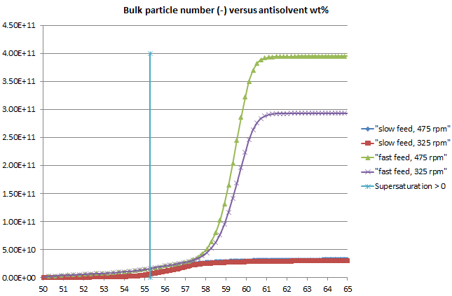
Figure 2: The number of particles formed in the system is higher when the addition rate is faster; this tallies with the higher level of supersaturation reached, with a greater driving force for nucleation. The simulation includes a direct effect of impeller speed on nucleation, leading to more particles at higher agitation speed (and fast addition).
Figure 3: In this model, the number of particles in the feed zone is tracked separately from those in the bulk; this number depends primarily on the quality of meso- and micromixing and there are more particles formed in the feed zone at lower agitator speeds. The number of particles in the feed zone is significantly higher with fast feeding. Note that particles are formed from the start of the addition but many of the 'oldest' dissolve in the bulk while those formed later have a better chance of remaining out of solution.
Figure 4: A plot of bulk particle number versus wt% antisolvent, with the scale reduced to highlight the first signs of particles in the bulk, indicates that a large number of particles may exist even when the system is undersaturated and the number of particles can be several times higher with fast feeding than with slow.
Such a particle number profile would make it more likely that a negative MSZW would be observed at higher addition rates when the FBRM (or other particle monitoring) probe may detect the larger particle number.
A potentially interesting parameter to complement MSZW is the observed induction time, which in the case of the present system reduces at higher addition rates and is often well under 1 second. This underlines the importance of rapid local mixing of the feed and induction time could be used to calculate a Damkoehler type number for the system.
The stochastic nature of both MSZW and induction time is well recognized and addressed again in a recent paper.
From a practical point of view, all of this makes it even clearer that relying on uncontrolled primary nucleation as a means to obtain a desired crystal size (or number) can be a risky approach. The same models shown here can be used to investigate the impact of seeding and to find more robust, growth-dominated conditions in a specific system.
Whatever about the quantitative and specific interpretation of the simulation results shown, the power to quickly visualize these potential impacts before experiencing them in practise is of great educational value and assists with experimental design and planning. Which reminds me of the poster I saw on the wall at a large chemical company several years ago, which read: "Don't speculate, Simulate!".